
伏隔核 (NAc) 是基底神经节回路的关键组成部分,它将来自皮质和边缘区域的信息整合到直接行为中。先前的研究表明,NAc 参与调节多种行为,包括食欲和厌恶反应、进食、社交互动、强化和工具学习。此外,临床和临床前研究已将 NAc 功能障碍与多种神经精神疾病联系起来,包括抑郁症、焦虑症、精神分裂症和药物滥用 。与其功能多样性一致,NAc 与不同的大脑区域建立了复杂的神经连接。越来越多的证据表明,NAc 的特定输入/输出回路可能是其不同功能的基础。
考虑到 NAc 的功能和解剖复杂性,对细胞组成和结构的理解仍然有限。一般来说,超过 90% 的 NAc 神经元是 GABA 能中等多刺神经元 (MSNs),中间神经元 (INs) 的比例很小。传统的直接/间接通路模型根据其基因表达、连接性和功能将 MSN 分为 D1 多巴胺受体表达亚型和 D2 多巴胺受体表达亚型(D1 和 D2 MSN)。
虽然该模型为理解纹状体的细胞和回路组织提供了一个框架,但它在很大程度上忽略了纹状体内的异质性,因此不能很好地解释 NAc 的解剖和功能多样性。例如,背侧纹状体 (DS) 中的纹状体/基质隔室和 NAc 中的核/壳组织表现出离散的分子和解剖学特征。此外,位于 NAc 不同甚至相同子区域的 MSN 与不同的上游和下游目标连接。此外,不同的神经功能被归因于不同的 NAc 亚区,甚至是近距离内的相同神经元亚型(例如,D1 MSN)。
Abstract
The nucleus accumbens (NAc) plays an important role in regulating multiple behaviors, and its dysfunction has been linked to many neural disorders. However, the molecular, cellular and anatomic heterogeneity underlying its functional diversity remains incompletely understood. In this study, we generated a cell census of the mouse NAc using single-cell RNA sequencing and multiplexed error-robust fluorescence in situ hybridization, revealing a high level of cell heterogeneity in this brain region. Here we show that the transcriptional and spatial diversity of neuron subtypes underlie the NAc’s anatomic and functional heterogeneity. These findings explain how the seemingly simple neuronal composition of the NAc achieves its highly heterogenous structure and diverse functions. Collectively, our study generates a spatially resolved cell taxonomy for understanding the structure and function of the NAc, which demonstrates the importance of combining molecular and spatial information in revealing the fundamental features of the nervous system.
Methods
data filtering and quality control
The R package Seurat (v2.1.0) and some customized R scripts were used for data analyses.
First, the expression matrices of all the 11 samples were pooled together into a global Seurat object using the MergeSeurat function.
1 | MergeSeurat(object1, object2, project = NULL, min.cells = 0, |
- Genes expressed in fewer than three cells were excluded.
- The cells with more than 10% of their total transcripts from mitochondrial transcriptome
cells with a large number of uniquely expressed genes (more than the 99th percentile, 4,766 genes) were removed.
For the initial analysis, all single cells expressing ≤1,500 genes were also excluded.
In total, an expression matrix including 19,458 genes and 37,011 cells was obtained. The gene expression profile of each single cell was then normalized to count per million (cpm) and natural log-transformed. To further exclude potential experimental variations, a linear model was generated by using the ScaleData function in Seurat to regress out the effect of (1) the number of detected UMIs in each cell, (2) the percent of mitochondrial genes and (3) sample-to-sample variation.
Separation of cells into neuronal and non-neuronal populations and detection of major cell populations
To detect the major neuronal and non-neuronal populations, 2,104 genes with cpm >1.5 and dispersion (variance/mean expression) larger than one standard deviation away from the expected dispersion were selected as variable genes using the Seurat function FindVariableGenes. The variable genes were used to calculate the top 30 principal components (PCs), and the significant PCs were selected using the JackStraw method in the Seurat package (P < 1 × 10⁻³). The cells were then classified into 25 clusters with the Seurat FindClusters function.
Then, the 25 initial clusters were merged using a random forest classifier with ten-fold cross-validation and 500 trees built with the caret R package, until the markers of each cluster had a strong predictive power (>80%), which led to 13 cell clusters.
Based on the expression of neuron-specific gene Snap25, the 13 cell clusters were identified as neuronal or non-neuronal clusters. In total, five neuronal clusters with 26,429 cells and eight non-neuronal clusters with 10,582 cells were detected.
These 13 major cell clusters were further aggregated into five non-neuronal populations (astrocytes, endothelial cells, microglia, oligodendrocytes and OPCs) and four neuronal populations (D1 MSNs, D2 MSNs, INs and new-born neurons) based on the expression of established marker genes, which is presented in Fig. 1.
Inclusion of non-neuronal cells with more than 800 genes detected
Previous studies showed that neuronal cells tend to have a higher number of mRNAs (UMI) and genes than non-neuronal cells, which is also confirmed in our dataset. Thus, the criteria used above (>1,500 genes detected) excluded many non-neuronal cells.
Hence, we decided to include non-neuronal cells with more than 800 detected genes, which was regarded as high-quality cells in previous high-throughput scRNA-seq studies. To this end, the cells expressing ≥1,500 genes were used to train a random forest classifier (500 trees and ten-fold cross-validation) to predict the identity of the cells expressing 800–1,500 genes. Only cells predicted as non-neuronal populations were included. This led to a dataset containing 26,429 neuronal cells and 26,913 non-neuronal cells.
Clustering analysis of each major clusters
To further cluster the major clusters, the variable genes for each major cluster were identified with the ‘FindVariableGenes’ function in Seurat.
In this function, genes were placed into 20 non-overlapping bins according to their average expression, and then a z-score between their dispersion (variance/mean expression) and the mean dispersion of the bin was calculated. The genes with the expression cpm >1.5 and dispersion ≥1 standard deviations away from the expected dispersion in the corresponding bin were selected as variable genes. In some cases, the threshold of dispersion was set to a higher value (up to 3 standard deviations) if the number of variable genes was greater than 2,500.
Then, the variable genes of each major cluster were used to calculate the top 30 PCs. Significant PCs with a P value of 1 × 10⁻³ were selected with the JackStraw method in the Seurat package. If too many PCs were significant, the top 10 PCs were selected.
After principal component analysis (PCA), the coordinates of the cells in the significant PCs were used as input for cell clustering. For each major cluster, we first forced the ‘FindClusters’ function to generate a large number of clusters by setting the resolution parameter to 3 or 4. Then, the marker genes of these clusters were calculated, and any pair of clusters with fewer than five DEGs (fold change >2 and P < 0.01) were merged.
Finally, we manually filtered out the cell clusters with substantial expression of
(1) neuronal and non-neuronal marker;
(2) established non-neuronal markers of different subtypes, because they potentially represent double droplets.
We also excluded the cell clusters expressing a high level of glutamatergic neuron markers (Slc17a6 and Slc17a7), because NAc does not contain glutamatergic neuron.
In addition, cell clusters contributed by cells from fewer than three samples were also excluded. After these processes, our pruned dataset included 25,734 non-neuronal cells and 21,842 neuronal cells.
Identification of cluster markers
The cluster-specific markers were identified by detecting the DEGs in the saline-treated samples by comparing their expression in the given cluster versus the other clusters. Specifically, the cluster markers were calculated by using a likelihood ratio test with an underlying negative binomial distribution (FindAllMarkers function of the Seurat package) while controlling for
(1) the number of UMIs in each cell;
(2) the percent of mitochondrial transcripts;
(3) sample-to-sample variation.
False discovery rates were corrected using the Benjamini–Hochberg method. The gene expression counts were assumed to follow a negative binomial distribution, but this was not formally tested. For MERFISH data, the two-sided, non-parametric Mann–Whitney test with Benjamini–Hochberg multiple testing correction was used (FindAllMarkers function of the Seurat package).
Figures
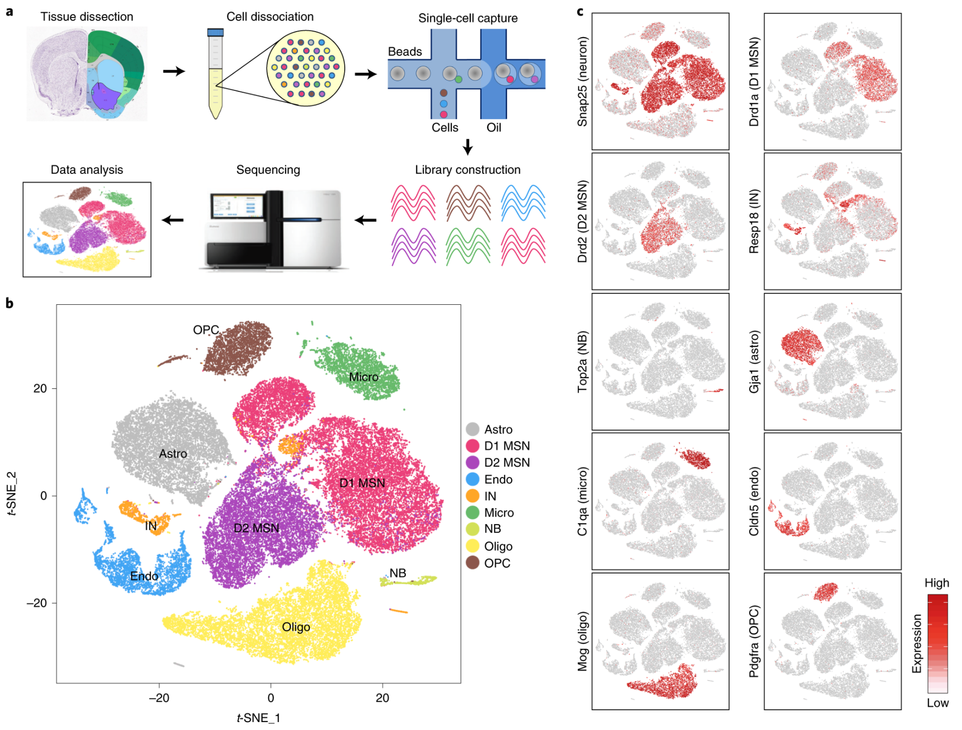
Fig. 1: scRNA-seq reveals major cell populations in the NAc.
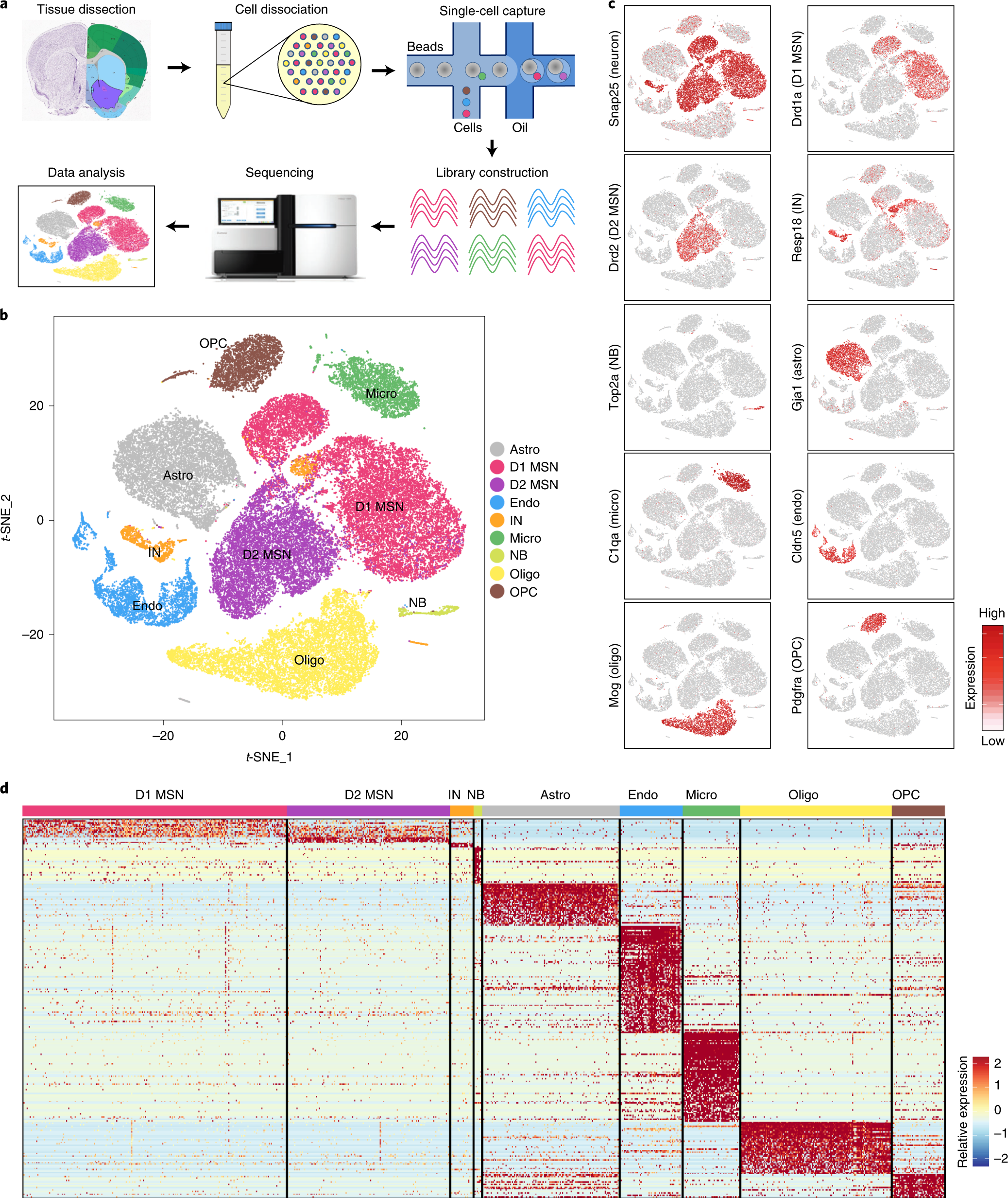
a, Workflow of scRNA-seq of mouse NAc. NAc tissues were dissected from adult mouse brain and dissociated into single-cell suspension. Single cells were captured into droplets with the 10x platform, followed by cDNA synthesis, amplification and library construction. After sequencing, cells were classified by their transcriptomes. b, t-SNE plot showing the different major cell types in the NAc. Different cell clusters are color-coded. c, t-SNE plots showing expression of cell-type-specific markers across different cell subtypes. The gene expression level is color-coded. d, Heat map showing that the cell-type-specific markers are differentially expressed across the nine NAc cell populations. DEGs with power >0.4 and fold change >2 among the nine cell clusters were used to generate the heat map. Columns represent individual cells, and rows represent individual genes. The gene expression level is color-coded. Astro, astrocyte; Endo, endothelial cell; Micro, microglia; NB, neural stem cells and neuroblasts; Oligo, oligodendrocyte; t-SNE, t-distributed stochastic neighbor embedding.
Fig. 2: Gene expression and spatial pattern of NAc IN subtypes.
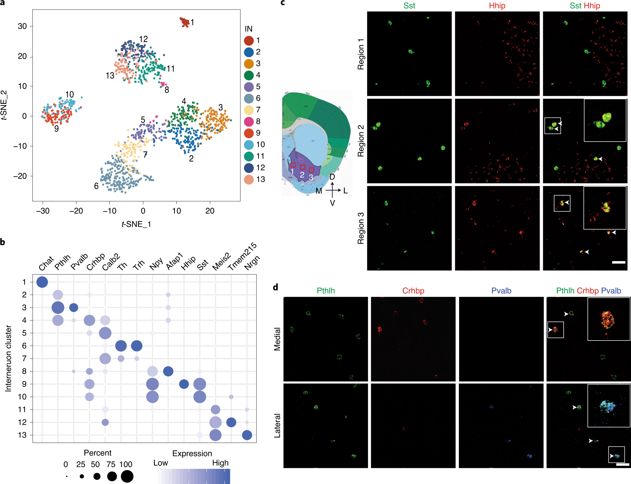
a, t-SNE plot showing the 13 IN subtypes identified in the NAc. DEGs among all subtypes are used for dimension reduction. Different neuron subtypes are color-coded. b, Dot plot showing the expression of selective markers in different NAc IN subtypes. The diameters of the dots represent the percentage of cells within a cluster expressing that gene. The gene expression level is color-coded. c, FISH showing the distribution of Sst+/Hhip+ and Sst+/Hhip− IN subtypes in different subregions of the NAc. The box regions labeled with 1–3 in the left panel indicate different subregions of the NAc (from medial to lateral), which are analyzed in the right panels (from upper to lower). The right panels show the FISH of NAc slice with Sst and Hhip probes. Arrowheads indicate cells co-expressing Sst and Hhip. Three independent experiments were performed with similar results. Scale bar, 100 µm. d, FISH showing the enrichment of distinct Pthlh+ IN subpopulations in different subregions of the NAc. The upper and lower panels represent the medial and lateral regions of the NAc. Triple-color FISH was performed with probes targeting Pthlh, Crhbp and Pvalb. Arrowheads indicate cells co-expressing Pthlh and Crbhp (upper panels) or cells co-expressing Pthlh and Pvalb (lower panels). Three independent experiments were performed with similar results. Scale bar, 50 µm. t-SNE, t-distributed stochastic neighbor embedding.
Fig. 3: Transcriptional features of MSN subtypes correlate with their spatial distribution in the NAc.
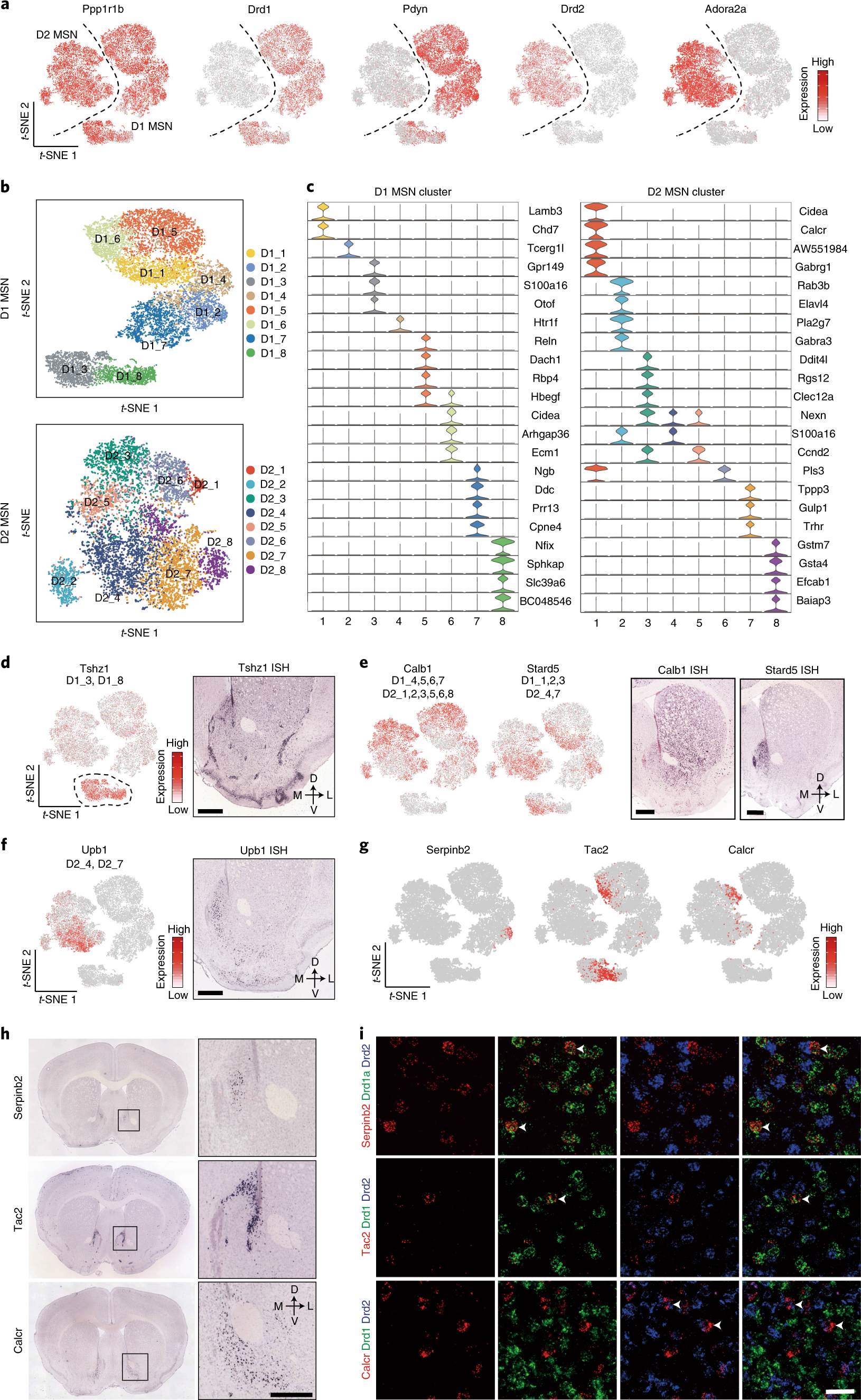
a, t-SNE plots showing the expression pattern of Ppp1r1b, Drd1, Pdyn, Drd2 and Adora2a in different MSN populations. The expression level is color-coded. b, t-SNE plots showing the eight D1 MSN subtypes (upper panel) and eight D2 MSN subtypes (lower panel); different subtypes are color-coded. c, Violin plots showing the expression pattern of MSN subtype-specific gene markers across the D1 MSNs (left) and D2 MSNs (right). Different MSN subtypes are color-coded. The mRNA level is presented on a log scale and adjusted for different genes. d, Tshz1 is enriched in a subpopulation of D1 MSNs. Left, t-SNE plots showing the expression pattern of Tshz1 across MSN populations. The expression level is color-coded. The MSN subtypes labeled by Tshz1 are indicated. Right, ISH of Tshz1 showing the distribution of Tshz1+ cells in the NAc. Coronal section of mouse brain including NAc is shown. Data were obtained from the Allen Mouse Brain Atlas. Scale bar, 500 µm. e, Calb1 and Stard5 showing anti-correlated expression pattern. Left two panels, t-SNE plots showing the expression of Calb1 and Stard5 as detected by scRNA-seq across D1 and D2 MSNs. The gene expression level is color-coded. The MSN subtypes labeled by Calb1 and Stard5 are indicated. Right two panels, ISH of Calb1 and Stard5 showing their anti-correlated expression pattern in the NAc. The ISH data are from the Allen Brain Atlas. Scale bars, 500 µm. f, Upb1+ D2 MSNs are distributed in the medial NAc. Left panel, t-SNE plot showing that Upb1 expression is restricted in certain D2 MSN populations. Right panel, ISH image showing the distribution of Upb1+ cells in the NAc. Data were obtained from the Allen Mouse Brain Atlas. Scale bar, 500 µm. g, t-SNE plots showing the expression of selected MSN subtype markers across MSNs. Transcriptional levels are color-coded. h, ISH images showing the spatial distribution of Serpinb2, Tac2 and Calcr, markers of certain D1/D2 MSN subtypes, in mouse NAc. Boxed regions in left panels are enlarged and shown in the right panels. The data are from the Allen Mouse Brain Atlas. Scale bars, 500 µm. i, Three-color FISH confirms the expression of MSN subtype-specific markers in the NAc. The arrowheads indicate cells that co-express selected MSN subtype markers with Drd1 or Drd2 in mouse NAc. Three independent experiments were performed with similar results. Scale bar, 50 µm. t-SNE, t-distributed stochastic neighbor embedding.
Extended Data Fig. 1: Identification of the transcriptionally distinct cell types in mouse NAc.

a, Schematic diagram showing the nucleus accumbens region used for single-cell RNA sequencing. Adult mouse brain was first cut into 0.5mm-thick serial coronal sections and then NAc tissues (shown in purple contours) were dissected from successive slices along the rostral-caudal axis. The brain pictures were taken from Allen Mouse Brain Atlas. b, Bargraphs showing the distribution of UMI and gene number detected in each cell across the 11 samples. Different samples are color-coded. The black central line is the median, the box limits indicate the upper and lower quartiles, the whiskers indicate the 1.5 interquartile range and dots represent outliers. c, Histograms showing the percentage of cells from each sample that contribute to the major cell clusters. Different samples are color-coded. d, Bargraphs showing the distribution of UMI and gene number detected in each cell across the 9 major cell clusters. Different cell clusters are color-coded. The black central line is the median, the box limits indicate the upper and lower quartiles, the whiskers indicate the 1.5 interquartile range and dots represent outliers. Astro, astrocyte; D1, medial spiny neuron, D1-receoptor subtype; D2, medial spiny neuron, D2-receptor subtype; Endo, endothelial cell; IN, interneuron; Micro, microglia; NB, neural stem cells and neuroblast; Oligo, oligodendrocyte; OPC, oligodendrocyte progenitor cell. e, ROC curves showing the high accuracy of the cell identity predictor, especially for non-neuronal cells. The curves of different cell types are represented by different colors. f, Heatmap showing the results of predicted identity of cells with 800 to 1,500 genes detected. The prediction probability is color-coded. g, In situ hybridization of the cell-cycle gene, Top2a, showing the distribution of neural stem cells and neuroblasts in the ventral wall of the lateral ventricle. The purple contour indicates the NAc, and the boxed region in the left panel is enlarged and shown on the right. The ISH data was obtained from Allen Mouse Brain Atlas. Scale bar, 100 µm.
Extended Data Fig. 2: Gene expression and spatial pattern of NAc interneuron subtypes.

a, Hierarchical relationship of the 13 NAc interneuron subtypes identified from scRNA-seq. The dendrogram indicate the relatedness among interneuron subtypes based on their gene expression. The markers and the number of cells of each subtypes are shown. b, Heatmap showing the expression pattern of interneuron markers across different subtypes. Each column represents a single cell. The gene expression level is color coded. The 13 interneuron subtypes are indicated by different colors on top. c, ISH showing the expression of selected interneuron subtype markers identified by scRNA-seq in NAc. The regions around the anterior commissure (AC) were shown except for Pvalb, which was more enriched in lateral part of NAc. The images were obtained from the Allen Mouse Brain Atlas. d, tSNE plots showing the expression of interneuron subtype markers across NAc interneuron subtypes. The gene expression level is color-coded. e, FISH showing the overlap of selected interneuron markers in NAc. Arrow heads indicate the cells co-express the two genes. Arrows indicate cells expressing one marker gene. Three independent experiments were performed with similar results. Scale bar, 50 µm.
Extended Data Fig. 3: Molecularly defined MSN subtypes exhibit distinct spatial distribution in NAc.

a, Histograms showing the percentage of cells from each of the 11 samples across D1 and D2 MSN subtypes. Different samples are represented in different colors. b, tSNE plots showing the expression pattern of Lrpprc, Foxp2, Foxp1 and Isl1 across MSN populations. The expression level is color-coded. c, ISH of Tshz1 showing the distribution of Tshz1+ cells in NAc. Sagittal section of mouse brain including NAc is shown. The boxed region is enlarged and shown on the right. Data are obtained from Allen Mouse Brain Atlas. Scale bars, 500 µm. d, e, Ddit4l (d) and Trhr (e) are enriched in subpopulation of MSNs. Left panel, tSNE plots showing the expression pattern of Ddit4l (d) and Trhr (e) across MSN populations. The expression level is color-coded. The MSN subtypes labeled by Ddit4l or Trhr were indicated. Right panels, ISH image showing the distribution of Ddit4l+ (d) and Trhr+ (e) cells in NAc. The boxed regions are enlarged and shown on the right. Data is obtained from Allen Mouse Brain Atlas. Scale bar, 500 µm. f, Heatmaps showing the gene expression correlation of differentially expresses genes in D1 MSNs (upper panel) and D2 MSNs (lower panel). The correlation is color-coded, and genes were sorted into groups with higher intra-group correlation. g, h, Violin plots showing the expression of selected markers across high-resolution D1 (g) and D2 (h) MSN subtypes. Different MSN subtypes are color-coded. The mRNA level is presented on a log scale and adjusted for different genes.
reference: